Excel for Finance: Step-by-Step Guide to Calculating YTM and Bond Price (Using IRR and PRICE Functions)

In high-stakes NISM technical examinations, time is your most precious resource. Manual calculation of complex financial metrics like Yield to Maturity (YTM) and Bond Price can be incredibly time-consuming and prone to error. Fortunately, Excel provides built-in functions that allow you to compute these values in seconds, enabling you to dedicate more time to challenging theoretical questions. This guide provides a hands-on, step-by-step approach to mastering these critical Excel functions.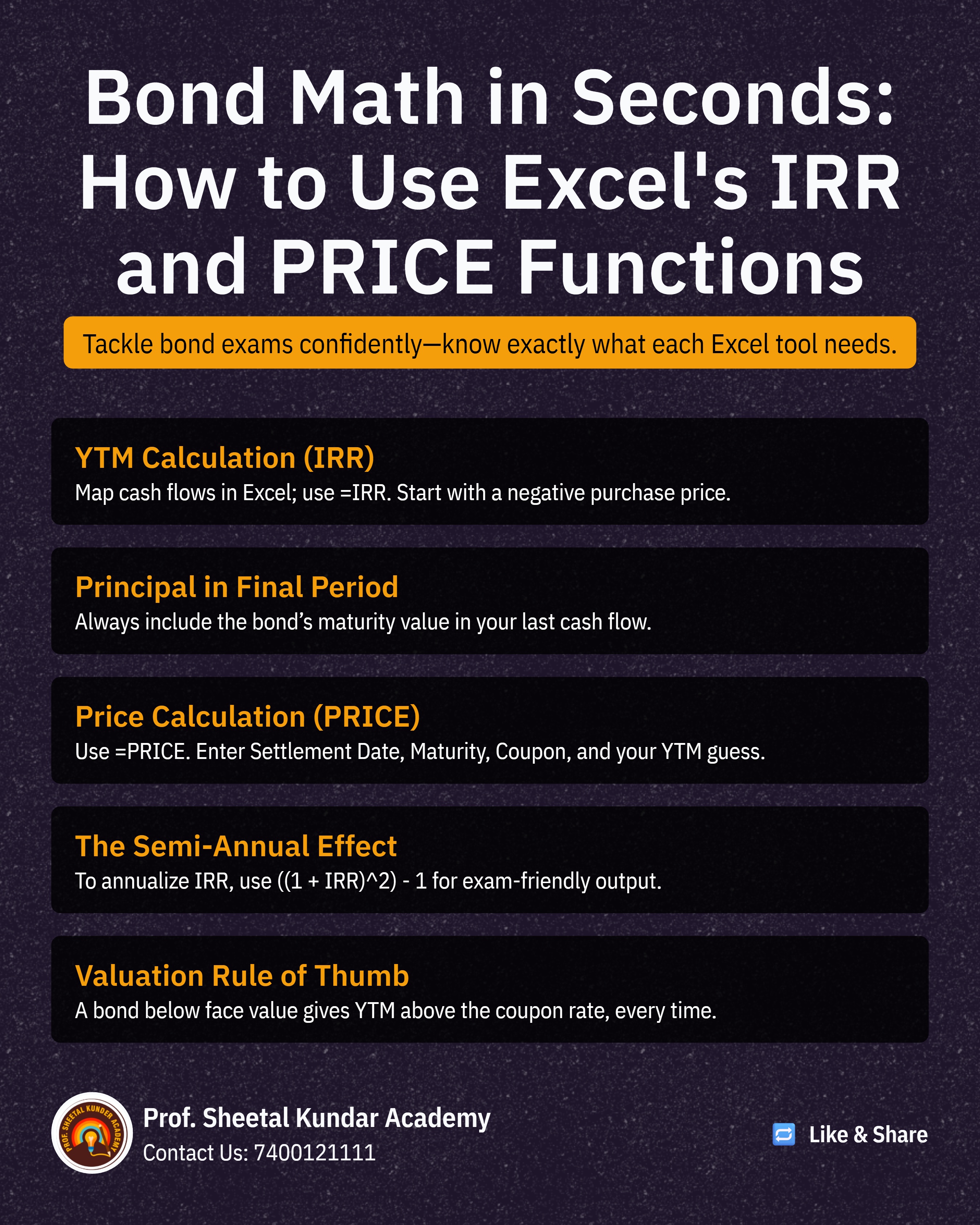

1. Calculating Yield to Maturity (YTM) using the IRR Function

YTM is the total return anticipated on a bond if it is held until its maturity date. It is calculated based on the bond's cash flows—coupons and the principal repayment—and is computationally intensive when done manually.

Scenario: A bond with a Face Value of ₹1,000, an 8% annual coupon paid semi-annually, a Purchase Price of ₹950, and 3 years to maturity.

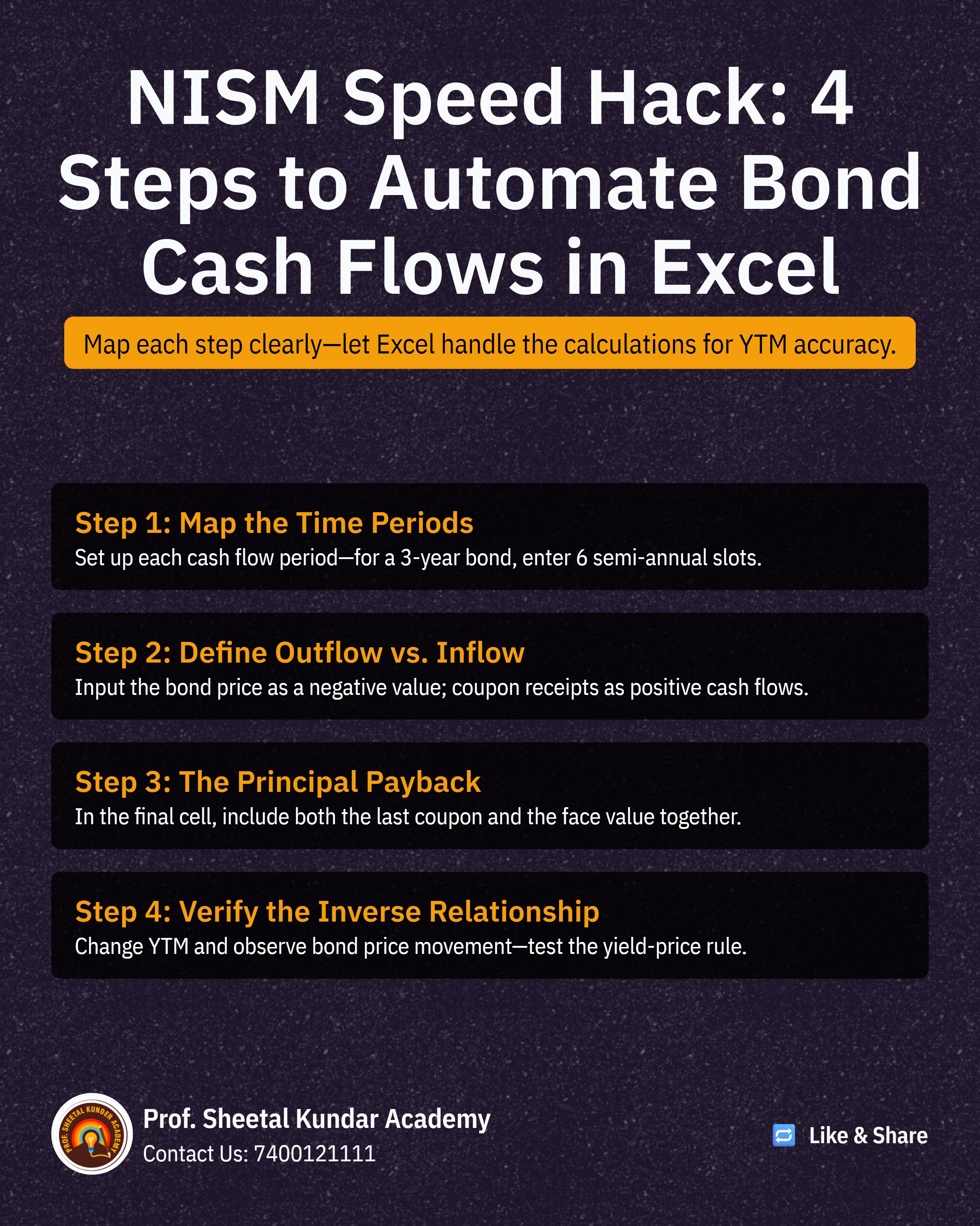
Steps to Calculate:

Map Cash Flows: Set up the cash flows across the relevant periods. Since the coupon is semi-annual and the maturity is 3 years, you have 6 periods.

Period 0 (Purchase): This is a cash outflow, so enter -₹950.

Periods 1 through 5 (Coupons): The annual coupon is 8%, so the semi-annual coupon is 4% of ₹1,000, or ₹40. Enter ₹40 for these 5 periods.

Period 6 (Maturity): The final payment is the Face Value plus the last coupon: ₹1,000 + ₹40 = ₹1,040.

Use the IRR Function:

In an empty cell, type: =IRR(

Select all cash flow values, from -₹950 to ₹1,040.

Close the bracket and press Enter. The result, approximately 4.985%, is the semi-annual rate

Annualize the YTM: Since NISM questions typically require the Annual YTM, you must convert the semi-annual rate using the following formula:

Type: =((1 + IRR_Result)^2) - 1

This will yield the annualized YTM (e.g., 10.22%), confirming that since the bond was bought below Face Value (₹950 < ₹1,000), the YTM is higher than the coupon rate (8%).

2. Calculating Bond Price (Bond Value) using the PRICE Function

The Bond Price, or Bond Value, determines what a buyer should pay for the bond given a target yield. This can be easily computed using the built-in PRICE function.

Scenario: Calculate the bond value given a 7% Annual Coupon, 7.50% YTM, and a redemption price of ₹100 (as a percentage of face value).

Steps to Calculate:

Use the PRICE Function:

In an empty cell, type: =PRICE(

The function will prompt you for a series of fields; the key is to ensure the dates and formats are correctly input.

Enter Key Fields:

Settlement Date: The date the bond is purchased (select the cell containing this date).

Maturity Date: The date the bond matures (select the cell containing this date).

Rate: The Coupon Rate (e.g., 7%).

YIELD: The target Yield to Maturity (e.g., 7.50%).

Redemption: The redemption value (usually 100 if it matures at par value).

Frequency: The frequency of coupon payments (e.g., 2 for semi-annual).

Result: Press Enter to get the Bond Price. You can then change the Coupon Rate or YTM inputs to instantly see the impact on the Bond Price, confirming the inverse relationship (higher YTM leads to lower price).

Mastering the IRR and PRICE functions for YTM and Bond Price computation is paramount. It allows you to swiftly handle numerical questions and verify theoretical concepts, thereby significantly boosting your confidence and speed in the NISM exam.